02

The loop

Takeaway. Self-play makes data, training updates the network, the new network plays better — repeat. Each cycle is one iteration.

• Self-play — the current network plays itself many times, choosing each move with MCTS.
• Buffer — every position $(s, \pi, z)$ is stored: state, MCTS visit distribution, eventual outcome.
• Train — minibatches from the buffer; loss has a value term, a policy term, and L2.
• Evaluate — the new network is checked against the previous best (AGZ) or simply adopted (AZ).

04

MCTS, with a prior

Takeaway. The network alone can only guess. Search lets the agent test its guesses by simulating moves forward — and the network makes the search dramatically more efficient by telling it where to look and how to score what it finds.

What is Monte Carlo Tree Search?

MCTS is a way to explore the future of a game by simulating it. Starting from the current board, it builds a tree of possible continuations and uses the results of those simulations to decide which move is actually best right now.

The name "Monte Carlo" is historical: classical MCTS picks random move sequences from a position, plays them out to the end (a rollout), and uses the random win/lose outcomes to estimate which moves are good. The randomness — like the dice tables of the Monte Carlo casino — gives the algorithm its name.

AlphaZero drops the random rollouts. When the search reaches a position it hasn't seen, the value network reads the position directly and says "I think this is +0.4 — slightly winning." No coin-flipping. Much faster, much more accurate. The policy network is used too, to suggest where the search should look first.

One simulation, four phases

Per move, AlphaZero runs ~600 of these simulations. Each one is the same four-step recipe:

How a child is picked: the PUCT rule

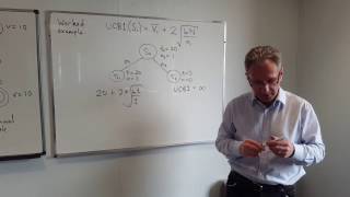
The interesting phase is Select. At every node, the algorithm has to pick which child to descend into. AlphaZero uses a formula called PUCT (Predictor + UCT) that scores each child by adding a "winning so far" term Q to an "exploration bonus" U:

$$ a^* = \arg\max_a \big[\, Q(s,a) \,+\, U(s,a) \,\big], \qquad U(s,a) = c_\text{puct} \cdot P(s,a) \cdot \frac{\sqrt{\sum_b N(s,b)}}{1 + N(s,a)} $$

Reading the terms one at a time:

• $Q(s,a)$ — the exploit term. The average value seen so far when the search picked move a from state s. If a led to good positions in previous simulations, Q is high. "This has worked."
• $P(s,a)$ — the network's policy prior. Probability that the network's policy head assigned to move a. Without this, the search would have to consider all 82 actions equally — most of which are obviously bad. "The network thinks this is promising."
• $N(s,a)$ — the visit count. How many simulations have already gone through this move. Appearing as a denominator, it makes already-explored moves less attractive — pushing the search to try things it hasn't seen yet.
• $\sqrt{\sum_b N(s,b)}$ — total visits to this state's siblings, taken under a square root. Standard UCT scaling; grows slowly with experience.
• $c_\text{puct}$ — exploration constant. Bigger = more exploration. Typical values are 1–2.

So U is big when the network said the move looked good (high P) but we haven't tried it much (low N). Q is big when we've tried the move and it worked. PUCT picks the child where Q + U is biggest — exploiting what's worked while occasionally trying the network's untested suggestions.

What the network buys the search

• The policy prior P replaces uniform exploration over the 82 legal actions. Without it, the search would waste most of its budget on terrible moves (placing in the centre on move 1, etc.).
• The value V replaces classical rollouts. Without it, every leaf would have to be evaluated by playing the rest of the game out randomly — noisy, slow, and in Go often misleading.
• Together: the search is guided by learned intuition and grounded by learned judgment. It looks where it should and scores what it finds.

What the search hands back

After all 600 simulations, the root has accumulated a visit count $N(s_0, a)$ for every legal move. The move distribution played by the agent is:

$$ \pi(a) \;\propto\; N(s_0, a)^{1/\tau} $$

where τ is a temperature (more on that in the next section). This π is the search-improved policy. Crucially, it is almost always better than the network's raw policy p, because the search has had a chance to look ahead and discard moves that looked good in p but turned out badly in simulation. That's why π — not p — is what the agent plays, and what the policy head is trained against.

A small worked example

Imagine the agent is about to make its very first move on an empty board. The network's policy head outputs probabilities — let's say it's slightly biased toward 3-3 and 4-4 corner points (the kinds of moves that tend to win, from training):

$P($corner 3-3$) = 0.15, \quad P($corner 4-4$) = 0.20, \quad P($centre tengen$) = 0.05, \quad …$

MCTS starts simulating. The first simulation can't use Q (nothing has Q yet — N is 0 everywhere), so PUCT reduces to "follow the network's prior." It picks 4-4. The search descends into 4-4, expands it, the network reads the resulting position and says V = +0.05 (slightly winning). That +0.05 is backed up. Now root's child 4-4 has $Q = 0.05$ and $N = 1$.

The next simulation re-scores all children. 4-4's exploration bonus dropped (because N is now 1). So PUCT might now pick 3-3 instead, expand it, get a value back, etc. Over 600 simulations, moves that consistently lead to high-value positions accumulate visits; moves that lead to losses get visited a few times and then ignored. The visit counts at the end are sharper and better-informed than the raw policy prior was.

Watch the search in action — and try building it

▶

Video · John Levine · 16 min

Monte Carlo Tree Search

The clearest visual MCTS walkthrough on YouTube. Uses tic-tac-toe to show all four phases. Used in many university courses.

▶

Video · DeepMind · 14 min

AlphaGo Zero: discovering new knowledge

A short overview from DeepMind on how AGZ bootstraps and what it discovers along the way.

▶

Video · David Silver lecture · 1 h 45 m

Deep Reinforcement Learning and AlphaGo

DeepMind's lead author walks through MCTS, the policy/value architecture, and how it all comes together. Long but worth it.

▶

Video · Robert Förster · 24 min

AlphaZero — Paper Walkthrough

A focused, accessible walkthrough of the 2018 AlphaZero paper. Reads the algorithm and the loss alongside annotated figures.

GitHub

AlphaZero
from scratch

code + tutorial

Code · GitHub repo + 4-video series

AlphaZero From Scratch (Robert Förster)

A clean, well-commented PyTorch implementation paired with a tutorial series. The best place to read the algorithm in code.

07

Pseudocode

Takeaway. Four pieces — outer loop, self-play game, MCTS search, training step — each fits on one screen. Click between tabs to read them as a connected whole.

# Outer loop — runs for N iterations
network ← random_init()
best    ← network
buffer  ← empty()        # replay buffer of (s, π, z)

for iteration in 1..N:

    # 1. self-play with the current best network
    for g in 1..games_per_iter:
        examples ← play_self_play_game(best)
        buffer.extend(examples)

    # 2. train a candidate on the buffer
    candidate ← network.copy()
    for step in 1..train_steps:
        batch ← buffer.sample(batch_size)
        train_step(candidate, batch)        → tab 4

    # 3. evaluate: AGZ gates by 55% arena win-rate; AZ adopts unconditionally
    if arena(candidate, best) ≥ 0.55:
        best ← candidate

    network ← candidate

# One self-play game
def play_self_play_game(network):
    state    ← initial_state()
    examples ← []
    move_num ← 0

    while not state.terminal():
        # run MCTS to get visit counts at this state
        N ← mcts_search(state, network)         → tab 3

        # temperature schedule: explore early, exploit late
        τ ← 1.0 if move_num < 30 else 0.0
        π ← N^(1/τ) / sum(N^(1/τ))

        # store the training example (outcome filled in later)
        examples.append((state, π, state.player))

        # sample and play an action
        a     ← sample(π)
        state ← state.play(a)
        move_num += 1

    # game ended — stamp every example with z from that player's view
    winner ← state.score()
    for (s, π, player) in examples:
        z ← +1 if winner == player else −1
        yield (s, π, z)

# MCTS search — the heart of AlphaZero
def mcts_search(root_state, network):
    root ← Node(root_state)
    # root prior + Dirichlet noise for exploration
    p, v ← network(root_state)
    root.P ← (1−ε)·p + ε·dirichlet(α)
    root.expand()

    for _ in 1..num_simulations:        # typically 600–800
        node, path ← root, [root]

        # PHASE 1: SELECT — descend by PUCT until leaf
        while node.expanded():
            a ← argmax_a [ node.Q[a] + c·node.P[a] · √(ΣN) / (1+node.N[a]) ]
            node = node.children[a]
            path.append(node)

        # PHASE 2 + 3: EXPAND + EVALUATE
        if not node.state.terminal():
            p, v ← network(node.state)
            node.P ← p
            node.expand()
        else:
            v ← node.state.terminal_value()

        # PHASE 4: BACKUP — propagate v up the path
        for n in reverse(path):
            n.N += 1
            n.W += v
            n.Q  = n.W / n.N
            v    = −v       # flip sign every level (opponent's turn)

    return root.visit_counts()

# One training step on a minibatch from the buffer
def train_step(network, batch):
    # batch contains (states, target_policies π, target_values z)
    states, π_target, z_target = batch

    # forward pass — network reads positions, predicts p and v
    p, v = network(states)

    # the AlphaZero loss has three terms
    value_loss  = mean((z_target − v)²)        # MSE on outcome
    policy_loss = −mean(sum(π_target · log(p)))  # cross-entropy on visit distribution
    reg_loss    = c · sum(θ² for θ in network.parameters())

    loss = value_loss + policy_loss + reg_loss

    # standard backprop + SGD update
    loss.backward()
    optimizer.step()
    optimizer.zero_grad()

    return loss.item()

• Self-play dominates wall-clock: each game requires hundreds of network forward passes per move.
• Training is fast — the network is small and the gradient step is standard.
• The arena gate (AGZ only) prevents bad updates from corrupting future self-play data.

08

AGZ → AZ

Takeaway. The 2018 AlphaZero paper drops three AGZ-specific tricks so the same algorithm works on chess and shogi. Otherwise identical.

Everything else — network shape, loss, MCTS-with-prior, self-play — is unchanged.

09

Training curve

Takeaway. Real data from our 6-iteration Connect Four run. After one iteration the full AlphaZero player already beats classical MCTS ~62% of the time; after six iterations it wins 96.5% and the bare policy network (no MCTS) reaches 46%.

For each iteration's checkpoint, we played 256 games against a fixed classical opponent — a Monte Carlo Tree Search with 1000 random rollouts per move. The opponent never changes, so the curve below is the actual strength of our agent over training time.

What the curve shows

• The full system learns fast. One iteration of training takes the AlphaZero player from 8.6 % to 62 % win-rate against a fixed MCTS opponent.
• The network alone learns slower. Without search, the policy head improves over time but trails the full system by roughly 50 percentage points. That gap is what MCTS is buying us at inference.
• Both curves rise together. The network's quality and the search's effectiveness aren't independent — better policy priors make MCTS more efficient; better-search-derived training targets make the policy better. This is the policy-iteration loop described in §06 in action.

Note on the y-axis: this first run plots win rate against a fixed external opponent (classical MCTS with 1000 rollouts) rather than Elo, because we had not yet configured per-iteration weight saving. Every later run did save its checkpoints — and §11 reports exactly the AlphaZero-paper-style Elo: round-robin tournaments between checkpoints, network sizes, search budgets and lesions, on both games, with confidence intervals.

Vs. the perfect solver (Pascal Pons)

The MCTS-rollouts opponent above is a strong baseline, but it is not optimal. To know how close to actual perfect play the agent gets, we benchmark it against the Pons solver — a famous open-source Connect Four solver that uses iterative deepening alpha-beta with a precomputed opening book, and which has been used as the de-facto perfect baseline for Connect Four AI research for nearly a decade.

One subtlety. Connect Four is a first-player win: if both sides play perfectly, white always wins. So the theoretical maximum win rate any agent can achieve against perfect play, over alternating-colour matches, is 50 % — winning all 50 as-white games and losing all 50 as-black games. The Pons opponent never makes a mistake, so as-black we lose every game; the only question is how well we play as-white.

What this tells us

• By iter 10, our 1.67-million-parameter network plays Connect Four optimally as the first player. Against a solver that knows every position perfectly, we win every single game in which we move first. Connect Four is a first-player win, so 50 % is the strongest possible result on the alternating-colour benchmark.
• The plateau is real, not a measurement artifact. The arena gate stopped accepting candidates after iter 10 — at the time we thought this was just noise. The Pons benchmark confirms: there is genuinely no room left to improve. The training did its job, then correctly stopped.
• ~10 iterations is enough. Connect Four is small, so this number doesn't transfer to bigger games (the original AlphaZero paper ran for hundreds of iterations on Go). But it does illustrate cleanly what "convergence" looks like in this kind of self-play loop.

10

Lesions

Takeaway. All four lesions measured against the perfect Pons solver. Removing search costs 29 points (50 → 21). Replacing the value head with classical rollouts is worse than removing search entirely — it costs all 50 points (50 → 0). Smaller capacity costs only 5 points.

The classic AlphaZero ablation question is: how much of the agent's strength comes from each component? We can answer it by degrading the agent one piece at a time and measuring the cost. We use the same iter-10 baseline network throughout (the converged checkpoint from the training curve), and play 100 games per arena against two opponents: RandomPlayer (uniform-random moves) and the Pons perfect solver.

Headline result: win rate vs perfect play

This is the chart that holds the news. Same network (iter 10) where applicable; same opponent (Pons); same 100-game sample size with alternating colours. The dashed red line at 50 % is the theoretical ceiling (Connect Four is a first-player win, so the best any agent can do over alternating colours is win all 50 as-white games and lose all 50 as-black games).

vs Random — saturated for everyone

Against a uniform-random opponent, all four variants (baseline, L1, L3, L4) win 100 / 100 games. Random is too weak to discriminate; you need a strong opponent like Pons to see the lesion costs. We mention the random-opponent number only to confirm that all variants are at least beating pure noise — the question is how they fare against perfect play.

Sims sweep (measured)

The classic AlphaZero compute curve plots strength against the number of MCTS simulations per move. We ran our iter-6 network against the same 1000-rollout MCTS opponent from the training curve, varying the trained agent's own MCTS budget from 2 to 600 simulations.

For reference, the same iter-6 network with sims ≥ 4 beats RandomPlayer 100 % of the time (with sims = 2 it still wins 88 %; see results/sims_sweep.csv). Random play is too weak to differentiate the search budget once it's non-trivial.

What each lesion teaches us

• L4 — capacity matters surprisingly little. The small network (93 k parameters, 18× smaller than the baseline) plays Connect Four almost as well as the big one: 45 % vs Pons compared to the baseline's 50 % ceiling. Connect Four is small enough that a tiny network can still represent the relevant patterns; the AlphaZero loop converges what it can. For a bigger game (9 × 9 Go), we expect this gap to widen.
• L1 — search is doing a lot of work, but not all of it. The bare policy network wins 21 % vs Pons — that's not nothing (random is 0 %), but it's far below the baseline's 50 %. About 30 percentage points come from MCTS at inference time, even with a perfectly good policy prior to start from. The network has learned to play Connect Four, but search is the second half of the algorithm.
• L3 — the headline negative result. The learned value head is irreplaceable. Drop just the value head — keep the policy prior, keep 600 MCTS simulations, keep everything else — and the agent wins zero games out of 100 against Pons. Including all 50 as-white games, where the agent has the inherent first-player advantage. Classical Monte-Carlo rollouts at the leaves are so noisy in Connect Four that they actively mislead a search guided by the correct policy. L3 is worse than L1. A trained value head is doing something fundamentally different and more useful than "many random simulations averaged together" — exactly the AlphaZero paper's claim.
• L2 — strength scales smoothly with search budget. From 2 to 256 sims, win rate rises roughly log-linearly (the canonical AlphaZero compute curve, Fig 6). The trained network amplifies its strength predictably with more thinking time. Below ~4 sims, search becomes worse than no search — too few simulations distort the policy distribution without giving useful look-ahead.

Ranked by Pons-benchmark cost

The cleanest one-line summary: when you compare against perfect play, the lesions rank like this from most-damaging to least:

11

9 × 9 Go

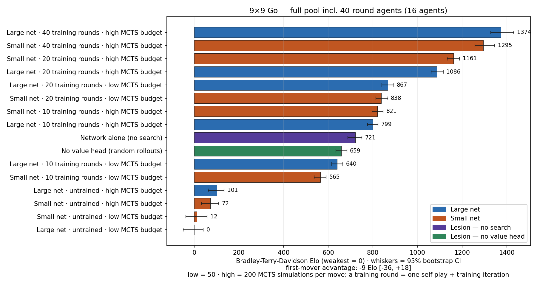
Takeaway. Stage two: we wrote a 9 × 9 Go rule engine for AlphaZero.jl, trained two network sizes from scratch on one GPU, and ranked 14 agent variants in a 9,500-game tournament. Training depth dominates everything (≈ +1,000 Elo from iteration 0 to 20). The Connect Four lesion ordering replicates. And a two-act surprise: at iteration 20 the 2.2× smaller network leads the pool — until doubling the training flips the order back to the big net (the epilogue below).

What we built

AlphaZero.jl knows nothing about Go. Everything the framework needs — legal moves, captures, ko, scoring — lives in one file we wrote, src/Go9.jl (~500 lines), implementing the GameInterface contract:

• Rules: standard placement and capture; suicide illegal; simple ko (a move may not recreate the board position from just before the opponent's last move); two consecutive passes end the game; Tromp-Taylor area scoring.
• Network input: a 9 × 9 × 4 tensor — own stones, opponent stones, a whose-turn plane, and a bias plane. All 8 board symmetries are exposed for training-data augmentation, exactly as AlphaGo Zero did.
• Three engineering choices that matter when reading the numbers below: komi = 0 (we keep the game symmetric for early training rather than compensating the second player; standard 9×9 komi is 5.5–7.5); simple ko rather than positional superko (rare long cycles are cut by a cap instead); and a 162-move safety cap (2 × board area), after which the board is scored as it stands. The cap binds in 12–13 % of games involving weak agents (untrained nets, classical rollout-MCTS) and essentially never between trained agents. Cap-terminated boards with large neutral regions are also the only realistic source of "draws" at komi 0.

Training two sizes from scratch

Both runs train on the same single GPU at roughly 45–60 min per iteration. Rule-engine sanity checks the framework can't do for us — ko handling, suicide masks, symmetry/policy consistency, scoring — are covered by scripts/test_go9_integration.jl and scripts/smoke_test_go.jl.

Does training work? Three independent yardsticks

• Against its own past. Iteration 20 beats iteration 0 50 : 0. In a five-way round-robin over iterations {0, 5, 10, 15, 20} (200 sims, 30 games per pair) every later checkpoint beats every earlier one; the narrowing 15-vs-20 margin (16 : 14) shows improvement flattening by iteration 20.
• Against classical search. The trained large net (200 sims/move) beats a vanilla MCTS using 1,000 random rollouts per move 30 : 0, and RandomPlayer 20 : 0.
• Search still scales. With the iter-20 net held fixed, every higher search budget wins its round-robin pairing: 16 < 64 < 200 < 800 < 3,200 sims (e.g. 3,200 beats 800 by 21 : 9). Unlike Connect Four — which our agent plays optimally by iteration 10 — 9 × 9 Go is nowhere near saturated: more thinking keeps helping.

The grand tournament — 14 agents, 9,500 games

The factorial design crosses 2 network sizes × 3 training stages (iter 0 / 10 / 20) × 2 search budgets (50 / 200 sims), plus the two lesions from §10 applied to the strongest large net: L1 (raw policy, no MCTS) and L3 (MCTS whose leaf values come from random rollouts instead of the value head). All 91 pairs play 100 games with colours strictly alternated, plus a 400-game per-colour calibration set. Ratings come from a Bradley-Terry-Davidson model (draws allowed) with a global first-mover-advantage term, fit jointly on all 9,500 games; uncertainty from 400 bootstrap refits of the entire tournament.

Four findings, with uncertainty

• Training depth dominates. Holding size and search fixed, going from iteration 0 to 20 is worth between +830 and +1,090 Elo depending on the size × sims cell. The single largest gap anywhere in the ranking is the +465 Elo [+421, +516] cliff separating the weakest trained agent from the strongest untrained one. Network size and search budget shuffle agents within a training stage; training moves them between stages.
• Search budget is the second axis. At iteration 20, 200 sims vs 50 sims is worth +222 Elo [+188, +258] for the large net (+318 for the small net). This matches the round-robin result above: on Go, unlike Connect Four, the compute dial keeps paying.
• The capacity surprise. The 2.2× smaller network is the strongest agent in the pool: +67 Elo [+31, +104] over the large net at the same iteration and search budget, P(stronger) = 1.00 — the ordering never reversed in 400 bootstrap refits. Strikingly, the ordering flips at low search: at 50 sims the large net leads by +30 Elo [−3, +63] (P = 0.96). So the bigger net evaluates single positions slightly better, but the small net profits more from search — consistent with its cheaper, possibly better-calibrated value estimates compounding over 200 simulations. One honest caveat: we trained one run per size. "The small net is at least as strong at this scale" is solid within this tournament; the stronger causal claim ("the large net is over-parameterised for 9×9") would need replicate training runs with different seeds — and in fact the catch-up epilogue below resolves it: with twice the training, the order flips back.
• The lesions replicate on a harder game. L1 (remove search, keep the trained policy) lands at 722 [693, 748] — a −368 Elo cost, equivalent to throwing away roughly half the training (it ranks between the iter-10 large net at 50 and 200 sims). L3 (keep search, replace the learned value head with random rollouts) is worse than no search at all: 660 [637, 686], i.e. −62 Elo below L1 [−94, −26]. On Connect Four L3 collapsed to 0 % against the perfect solver; on Go the penalty shows as a deficit rather than a collapse — there is no perfect opponent here to punish every misled line, but the ordering L3 < L1 < full agent is identical. A trained value head is not interchangeable with "average many random playouts". (With one instructive exception: in Connect Four pool play the order flips, because short-game rollouts carry real signal against imperfect opponents — see the Connect Four tournament below.)

Was colour handled fairly? (komi = 0)

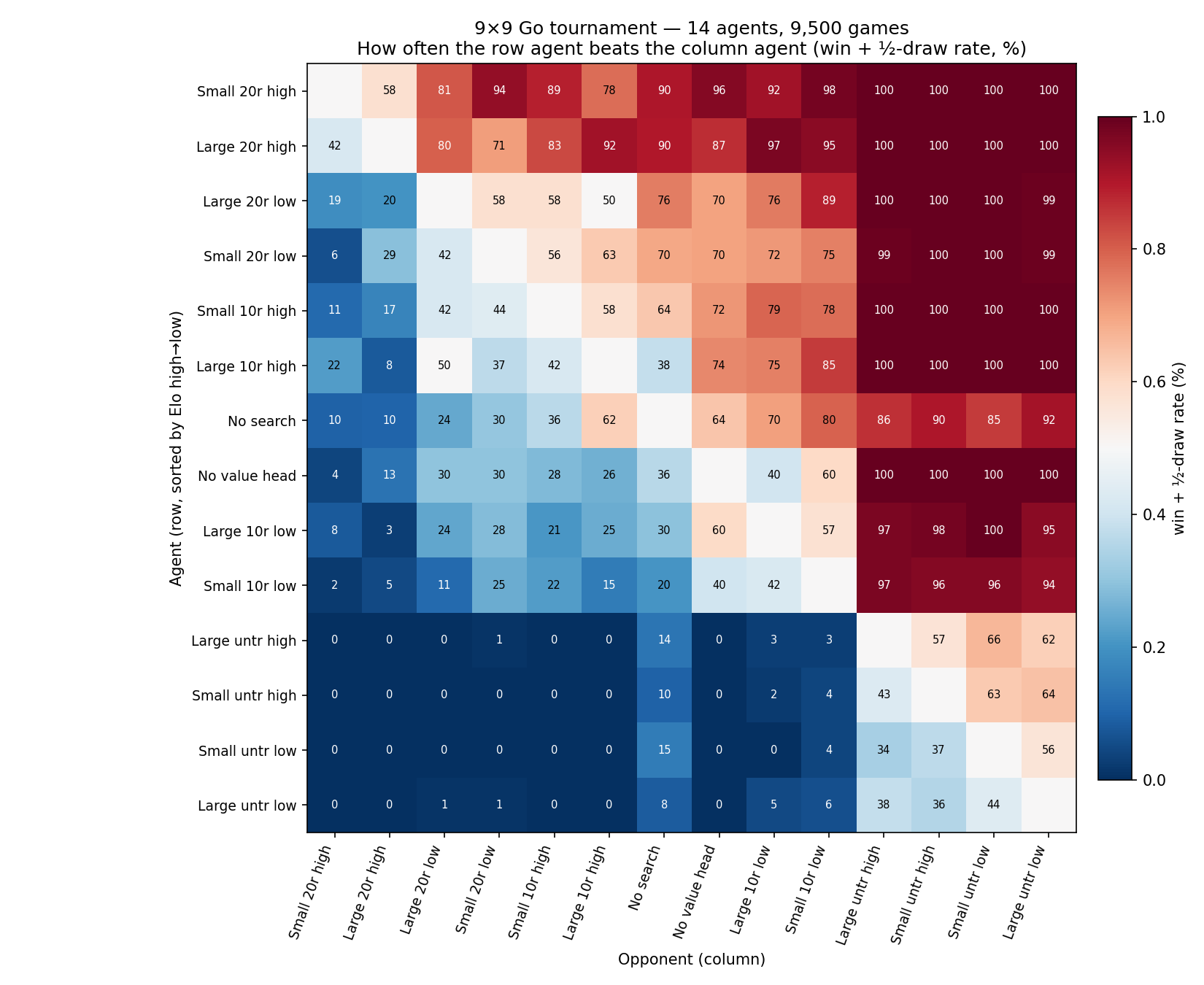
Two safeguards, one direct measurement. Design: within every 100-game pairing the colours strictly alternate — each agent plays exactly 50 games as first player and 50 as second — so no entry in the ranking ever compares agents at unequal colour exposure. Measurement: a separate 400-game calibration set recorded outcomes per colour; across it, the first player won 201 decided games and the second 198 (1 draw). Fitting a global first-mover term jointly on all 9,500 games gives +6 Elo [−46, +54] — indistinguishable from zero. This is itself informative: at komi 0, perfect 9×9 play is a first-player win (that is why real Go pays the second player 5.5–7.5 points of komi), so the absence of any measurable first-mover edge says our agents are still far from the regime where the first move can be converted reliably. If training is pushed further, this number should grow — and komi should be raised to ~7 before then.

Epilogue — double the training, and the big net passes

The capacity surprise begged a question: is the large net too big for 9 × 9 Go, or merely under-fed at 500 self-play games per iteration? The Connect Four flip below suggested the latter. So we doubled the training — both nets from iteration 20 to 40 (≈33 GPU-hours) — and ran a focused per-colour benchmark: each iteration-40 net against the other, against its own iteration-20 self, and against the other's iteration-20 self. 100 games per pairing, colours alternated.

Refit jointly over all 10,000 Go games, the final ranking puts large net, iteration 40, at 1,374 Elo [1,328, 1,431], ahead of small net, iteration 40, at 1,295 [1,258, 1,346] — with the iteration-20 ordering (small first) preserved below them. The capacity story completes: at matched, modest data the small net wins; give the big net twice the data and it overtakes, while the small net's returns flatten. Capacity isn't wasted on 9 × 9 Go — it just has to be paid for in self-play games. (The first-mover advantage, refit on 500 more per-colour games, tightens to −9 Elo [−36, +18]: still zero. And in 500 games between trained agents there was not a single draw — consistent with draws being a weak-agent, move-cap artifact.)

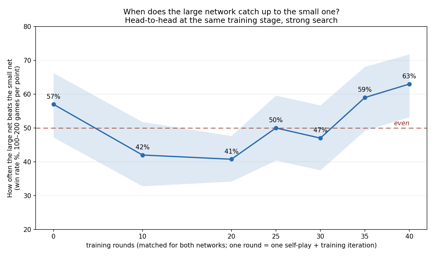
And when, exactly, did it catch up? Every training round was checkpointed, so we can ask directly: matched-stage duels every five rounds (100 games each) trace the whole arc. Untrained, the two nets are statistically even. Through rounds 10–20 the small net leads — the large net wins only 41–42 % of games. At rounds 25–30 they are back to even (50 %, 47 %). By round 35 the large net is ahead (59 %), and by 40 clearly so (63 %). The crossover sits around rounds 25–30 — roughly 12,500–15,000 self-play games before the extra capacity started paying rent. The early dip is the most instructive part: in the low-data regime the extra parameters actively hurt before they help.

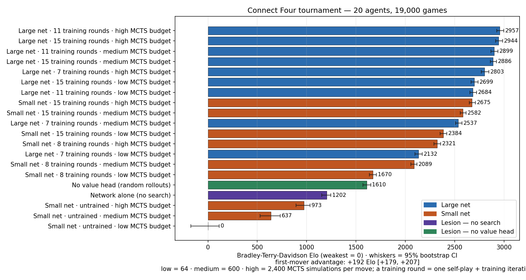
The same tournament on Connect Four — and two reversals

For symmetry we ran the identical design back on Connect Four: 2 network sizes (1.67 M vs 93 k parameters) × 3 training stages × 3 search budgets {64, 600, 2,400 sims} + L1 + L3 — 20 agents, 190 pairs, 19,000 games, with per-colour outcomes recorded for 114 pairs. Full ranking and pairwise matrix: results/tournament_c4_ranking_v2.png, results/tournament_c4_heatmap_v2.png. Read next to the Go results, three things stand out:

• Capacity flips back. On Connect Four the big net wins everywhere: at iteration 15 it leads the small net by ~270–300 Elo at every search budget (2,944 vs 2,675 at 2,400 sims; 2,886 vs 2,582 at 600; 2,699 vs 2,384 at 64). One reading consistent with both games: C4 training fed the network 5,000 self-play games per iteration, ten times Go's 500 — capacity pays off when self-play data is plentiful relative to model size, and Go's larger net may simply be under-trained for its parameter count rather than "too big". (Testing that would mean longer Go runs or richer self-play budgets.)
• First-mover advantage: +192 Elo [+179, +207] — about a 75 % win probability between equal players, draws aside — versus +6 Elo [−46, +54] on Go. Connect Four is a proven first-player win and our near-optimal agents convert that advantage relentlessly; our Go agents are nowhere near strong enough to exploit the first move at komi 0. Same model, same measurement, two regimes — and a live demonstration of why strict colour alternation inside every pairing is non-negotiable.
• The lesion ordering inverts in pool play. Against the perfect solver, L3 (random-rollout values) was catastrophic (0 %) while L1 (no search) salvaged 21 %. Inside the all-imperfect tournament pool the order flips: L3 (1,610) towers over L1 (1,202) by +408 Elo [+357, +463] — 81 : 8 in their head-to-head. Short Connect Four rollouts carry genuine signal, enough to out-calculate imperfect opponents; they only turn fatal against an opponent that punishes every rollout-induced error. On 9 × 9 Go, where games run to 162 moves over 81 points, rollouts are so uninformative that L3 falls below L1 even in pool play (above). So the value head's irreplaceability is regime-dependent: it matters most when games are long (rollouts become noise) or opposition is strong (errors become fatal) — and 9 × 9 Go is already in that regime.
• The tournament independently re-detects convergence. Iterations 11 and 15 are statistically tied (+13 Elo [−16, +44] at 2,400 sims) — echoing the Pons-solver finding that the network hit its ceiling around iteration 10 — while iteration 7 → 11 is still worth ~120–150 Elo. Search keeps paying even at the ceiling: 600 → 2,400 sims buys +58 Elo for the converged large net.